Proteomics mass spectrometry holds unlimited potential for translational “bench-to-bedside” medical research, but until now it lacked 3 must-haves: robustness, sensitivity, and verifiability. Clinical impact requires dependable analysis on low abundance peptides/proteins, with results that can be directly traced back to raw data. In contrast, most labs process data with low-priced or academic proof-of-concept software that lack some if not all of these requirements.
Here we address low-abundance and/or modified peptides (LAMPs). Specifically, we illustrate how to use the SORCERER GEMYNI data-mining platform to find, characterize, and quantify LAMPs in the intact peptide (“MS1”) mass spec data.
Our internal studies suggest: (1) LAMPs are distributed throughout MS1 data, (2) many exist for a split-second and are captured in a single MS1 scan, and (3) those exhibiting two isotopic peaks allow estimation of charge, intact mass, and rough peptide length. If SILAC light/heavy pairs are also identified, their number of ‘K’ and ‘R’ amino acid residues can also be inferred.
If you want something done right, do it yourself. A true “platform” lets you customize visualization and manipulation, which is critical for leading-edge research. No one but the scientists themselves can comprehensively analyze their own data.
Data-mining mass spec data is like analyzing a tiny drop of pond water with a powerful microscope — the deeper you look the more you see. In contrast, using a canned PC program is like being told by someone else what’s in your sample. You don’t learn as much and have no direct way to verify results.
Chromatography and mass spectrometry remain tricky yet doable, but the X-Factor is in data analysis as noted by the title of Scott Patterson’s 2003 paper (“Data Analysis – the Achilles heel of proteomics”, Nature Biotech)[1].
Basics of MS1 data
In shotgun proteomics, the first stage of a tandem mass spectrometry measures the mass/charge (m/z) ratio of peptides from an enzyme-digested protein mixture. This “MS1” data comprises triples of (scan#, m/z, intensity), which may also include the chromatographic retention time associated with the scan#.
Contrary to common preconception, MS1 data are quite easy to analyze at least in principle, but complex in practice due to overwhelming volume and overlapping peaks.
Raw MS1 data-points from the MSV000079761, a SILAC Yeast mzXML file available from ProteomeCommons[2]:
 scan  r-time    m/z     intensity
 ----- ------- -------- ------------
 18484 7120.63 448.7656      0.0000
 18484 7120.63 448.7692  28047.1641
 18484 7120.63 448.7728 175944.5938
 18484 7120.63 448.7764 420176.2812
 18484 7120.63 448.7800 632575.6875
 18484 7120.63 448.7836 661858.8750
 18484 7120.63 448.7871 484415.1875
 18484 7120.63 448.7907 230600.1250
 18484 7120.63 448.7943  53462.0352
 18484 7120.63 448.7979   6120.7920
 18484 7120.63 448.8015      0.0000
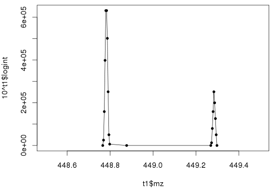
Figure 1: Intensity vs. m/z for two peaks
Figure 1 plots the above abundant peak (centered at m/z=448.7836) plus another (m/z=449.2833). The delta-mass of 0.5003 m/z suggests the peaks are isotopes of charge +2.
This means the intact mass is roughly 2*(448.7836 – 1.00278) + 1.00278, or 896.5644 amu.
Their peak ratio is 237K/662K = 0.36. A useful rule of thumb is that this ratio is roughly equal to the number of carbons divided by 80[3], especially if the peptide doesn’t contain sulfur. So there may be roughly 0.36*80 or 29 carbons. If we assume 4.9 carbons/residue on average, then the peptide is roughly a 6-mer.
To recap, with just two isotopic peaks from a single MS1 scan, we can estimate the charge, intact mass, and rough peptide composition. This information can potentially be used as a “peptide mass fingerprinting” (PMF) to supplement a standard proteomics workflow, for example to double-check protein quantitation.
Distribution of MS1 peaks
Using “log10(Intensity)” instead of “Intensity” is easier when working with LAMPs. Figure 2 shows the log(Intensity) version of Figure 1.
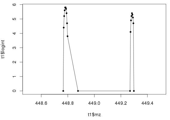
Figure 2: Log(Intensity) vs. m/z
Figure 3 shows the distribution of “Log10(Intensity)” for about 100 MS1 scans, which shows an asymmetric Gaussian-like distribution. Since we expect the number of peptides with Log(Intensity)<4.5 to be far higher than shown, we hypothesize the distribution is shaped by both instrumentation limitation (left-side) and the distribution of peptides in the sample (right-side).
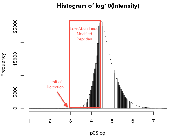
Figure 3: Distribution of Log(Intensity) from roughly 100 MS1 scans
Here, for practical consideration, we define LAMPs in terms of the instrumentation capability instead of absolute quantity, since we are interested in sensitive analysis not precise terminology. In other words, a peptide can be difficult for mass spectrometry due to low abundance or chemical modification.
The significance of the distribution is that we expect robust m/z and peak intensity only for log(Intensity) > 4.5. Below this point, accuracy may be compromised, or the peak may not be captured at all. We can test this by looking at data.
Map view of (r-time, m/z, logInt) triples
Instead of plotting on continuous axes of r-time and m/z (for example with heat maps), we find it useful to put “log(Intensity)” into a giant table where rows and columns are m/z and r-time, respectively. (To avoid the decimal point, the printed value is 10*log(Int), so “45” means log(Int)=4.5.)
Therefore, the following shows 4 abundant peaks spanning 23 seconds representing SILAC light/heavy pairs, which clearly suggest +2 charged peptides. A 5 m/z light/heavy separation with +2 charge suggests a single R in the peptide. Their SILAC quantitation ratio is approximately 1, which is expected for most SILAC light/heavy pairs.
                     rt=7107.64 to 7130.73 (9 scans)
                      -----------------------------
 454.3011[ 9666](  2):             42
 454.2975[ 9665](  8):    42 48 48 49 48 45 42
 454.2938[ 9664](  7):    47 52 52 53 52 50 46
 454.2901[ 9663](  7):    49 54 54 54 53 51 48     HEAVY SILAC (mono+0.5m/z)
 454.2865[ 9662](  8):    49 54 54 54 54 51 47     <--- Center at 454.2865
 454.2828[ 9660]( 11):    48 52 52 52 52 49 44
 454.2792[ 9658]( 12):    44 49 48 48 48 45
 454.2755[ 9656]( 10):       41       38
 .
 .
 .
 453.8003[ 9589](  6):    39 40 43 39 42 41
 453.7967[ 9588](  7):    48 50 52 51 51 49 45 41
 453.7930[ 9586](  8):    52 55 56 56 55 53 50 47
 453.7893[ 9584](  7):    54 57 58 58 57 55 52     HEAVY SILAC (monoisotopic)
 453.7857[ 9583](  7):    55 57 59 58 57 55 53     <--- Center at 453.7857
 453.7820[ 9580]( 10): 48 54 56 57 57 56 54 51
 453.7784[ 9579]( 15): 45 50 53 54 54 53 50 47
 453.7747[ 9577]( 32): 41 42 47 48 46 45 45 41
 453.7711[ 9576]( 21):                   44
 453.7674[ 9574]( 17):                   41
 .
 .
 .
 449.2977[ 8982](  2):                35 38
 449.2941[ 8981](  7):    40 47 46 47 48 46 40 36
 449.2905[ 8979](  8):    47 51 51 51 53 51 48 44
 449.2869[ 8978](  8):    49 53 54 53 55 53 51 46  LIGHT SILAC (mono+0.5m/z)
 449.2833[ 8977](  9):    50 54 54 54 55 53 51 46  <--- Center at 449.2833
 449.2797[ 8976]( 13):    49 52 53 52 54 52 50 44
 449.2761[ 8975]( 15):    45 49 50 49 50 48 46
 449.2725[ 8974]( 20):       43 42    41 42
 .
 .
 .
 448.7979[ 8926](  5):       37 32 38 37 39
 448.7943[ 8925](  7):    42 47 48 47 49 46 43
 448.7907[ 8924](  8):    49 52 54 54 54 53 50 46
 448.7871[ 8922](  8):    52 55 58 57 57 56 53 50  LIGHT SILAC( monoisotopic)
 448.7836[ 8921](  7):    54 56 59 58 59 57 54 51  <--- Center at 448.7836
 448.7800[ 8919](  8):    54 56 58 58 58 57 54 51
 448.7764[ 8917]( 10):    52 54 57 56 56 55 52 49
 448.7728[ 8916]( 11):    48 49 53 52 52 51 48 46
 448.7692[ 8915](  4):             44
Map showing LAMPs
When we map out a slightly larger slice of the (rtime, m/z) space, we see a multitude of single-scan runs of typically five 40-something values. (Enlarge Figure 4 PDF image for details.) This 5 m/z wide slice includes astonishing complexity.
That these runs are consistent in value and shape of peptides, and that occasional isotopic pairs are present suggest these are the elusive LAMPs.
We are unaware of prior reports of their existence in the MS1 data.
Indeed, LAMPs are generally invisible to conventional proteomics workflows geared toward abundant peptides. Their fleeting nature means they don’t appear in both MS1 and MS2 scans. As well, many workflows (e.g. SILAC) specifically average multiple scans.
msv_map
Figure 4: Peak map in PDF form showing many likely LAMPs (click to view)
2 Comments
Leave your reply.